The Importance of Shortwave Troughs and How to Identify Them

With the severe weather season upon us, I thought I would revisit and update an old post I wrote before joining Weather5280.
Shortwave troughs are features in the general flow of the atmosphere that are very important when it comes to forecasting, particularly for convective features and winter weather. Shortwaves can be thought of as "weather-makers," whereas Longwaves (Rossby Waves) might then be "trend-makers." Multiple shortwave troughs can be imbedded within a Rossby Wave trough. Shortwave troughs tend to move faster than their longer wavelength counterparts.
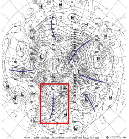
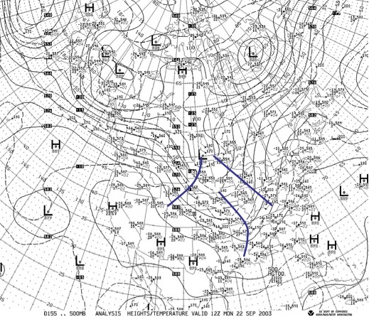
The images below are from a 500mb analysis at 1200 UTC 22 September 2003. The first image shows 6 longwaves around the Northern Hemisphere denoted by the blue lines across each long-wave trough axis. The second image depicts the 500mb analysis across North America only. Embedded within the Rossby Wave trough across the central US are 3 shortwave troughs moving around it, denoted by blue axes.
Here is a quick table to show the differences between Longwaves and Shortwaves. This table is assuming the observer is at 40° latitude.
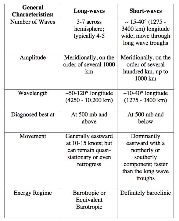
*At 40° latitude, 1° longitude ~ 85 km and at 45° latitude, 1° longitude ~ 79 km.
Identifying a shortwave trough in mid-levels of the troposphere is not always simple or straight forward, especially during the warm season (May-September). Here are some tips to help one identify shortwave troughs.
- Look for a trough in the height field. In the cold season, shortwave troughs are usually easily diagnosed through a good contour analysis. In the warm season, you may need to decrease the interval between heights to better define the trough (i.e., using a 30 gpm interval at 500mb instead of the standard 60 gpm).
- Locate a wind shift across the trough axis. Normally, winds should back as the shortwave trough approaches an area and then veer after passage of a trough. A 12 hour wind shift change can be used over a station to help individuals spot these trends.
- Analyze the isotherm pattern. Isoplething isotherms at a 2ºC interval on upper-level maps can help one spot subtle cool pools or thermal troughs that may not show up in the height analysis. Remember, heights of pressure surfaces are based on the mean temperature of the atmospheric column. Shallow cool pockets of air aloft may be masked by the height field since it is more sensitive to the mean temperature and not the level of analysis' temperature.
- Look at the mid-level dew points or dew point depressions. Downstream from the shortwave trough, you should observe higher dew points and lower dew point depressions than upstream from the trough axis. This assumption is based on the fact that there is generally upward vertical motion (UVM) downstream from the trough axis and downward vertical motion (DVM) upstream from the trough axis.
See the 500mb map from above for an example.
- Review the surface cloud reports. Typically, SW troughs aloft create mid-level cloudiness (i.e., altocumulus, altostratus, altocumulus castellanus) downstream from the trough axis. This is associated with mid-level UVM associated with the shortwave trough.
See the Visible satellite imagery from above for an example.
- Look at visible (VIS) and infrared (IR) satellite imagery. As noted in point (4), mid-level clouds are associated with shortwave troughs.
- Analyze the water vapor (WV) channel. Often jet streaks can be found coming around the base of a shortwave trough. This feature may show up as a dark slot on the WV imagery.
- Review a sounding. Soundings downstream from the shortwave trough should show a middle tropospheric layer of higher dew points and low dew point depressions even if clouds are not seen in the satellite imagery or surface cloud report.
- Look for a vorticity maximum, or "lobe" (elongated curved region) of vorticity. As noted in point (2), shortwave troughs have cyclonic wind shifts across their axis, which will show up on a vorticity analysis. Remember, when performing vorticity analysis, be sure to use absolute vorticity and not relative vorticity.
- Analyze the height change field (isallohypses). Similar to a frontal passage where an incoming front will have lower pressure tendency values ahead of it, the height field ahead of an approaching shortwave trough should have negative values in the isallohypses field.
I hope these basic pointers about short-wave trough identification will help you to become a better weather analyst. How many short-waves do you see in the image below?